Experiments on Topic Modeling – LDA

Topic modeling is an approach or a method through which a collection is organized/structured/labeled according to themes found in its contents. A more formal description would be that “topic models are a suite of algorithms that uncover the hidden thematic structure in document collections. These algorithms help us develop new ways to search, browse and summarize large archives of texts.”(quoted from David Blei, accessed Dec 12, 2017)

Topic modeling can be used in cluster analysis and that is the main reason why I wanted to understand how it works. It is based on the idea of a collection as a set of documents, which in their turn are made of words. Documents that are made of a certain group of words are likely to represent or belong to a certain topic. Words that are seen usually together are likely to constitute a topic. The frequency with which each word appears in relation to other words in a given document (inside a collection) is what constitutes the core of topic modeling.

Latent Dirichlet Allocation (LDA) is the simplest possible topic model. The intuition behind it is that a document can belong to multiple topics – just like a blog post can be archived under many different categories or with different tags. The graphic below (taken from the paper ‘Probabilistic Topic Models’, by David M. Blei) illustrates this intuition. Each color represents a topic.

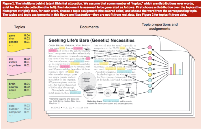
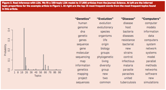
The graphic above illustrates what constitutes a topic: the words that occur more frequently (together) and thus can indicate a topic. The chart on the left indicates the inferred topic proportions in the documents collection.

Extracting topics from our data

In order to understand by doing, as a first step I decided to use the patents dataset as the collection from which to extract topics. There are many different modules (such as gensim, scikit) and methods (like LDA, NMF) to do that (as a reminder: Lídia and I have been using Python to explore and analyse data). All these possibilities can be quite challenging to someone who does not have a solid understanding of the statistical concepts that drive the technique, as the different ways to execute this task might be signaling that many factors play an important role in how it is executed. I opted to start by using Python’s LDA package, which is called as follows.

lda.LDA(n_topics, n_iter=2000, alpha=0.1, eta=0.01, random_state=None, refresh=10

The method requires six parameters, from which at least one must be specified, i.e., n_topics. The other 5 parameters, if not explicitly declared, will be the default values – the ones indicated after the equal sign in the code above. Here is a brief definition of the parameters:

• n_topics – number of topics to be extracted
• n_iter – number of sampling iterations
• alpha – Dirichlet parameter for distribution over topics
• eta – Dirichlet parameter for distribution over words
• random_state – the generator used for the initial topics
• refresh – when to update the model

First attempt

The dataset for this initial test is the patents titles. Using the patents extended description was consuming too much time (the corpus is many times bigger) so using a smaller dataset seemed a better idea. I experimented with the default values for all parameters and started by extracting one topic. One topic makes no sense in the context of topics extraction, but I was curious to see what group of words would be the most representative of Facebook’s patents titles – in a way, they should summarise what Facebook is most interested in or what Facebook does (since the data comes from patents granted to them). Here is the result:
1 topic, 2000 iterations, 7 words
Topic 0
['social' 'based' 'user' 'networking' 'systems' 'methods' 'content']

I chose to display the 7 most frequent words because the resulting list is not overwhelmingly long and it seems to provide a good overview of the topic. If, instead, I had chosen the 20 most frequent words, the result would be:
1 topic, 2000 iterations, 20 words
Topic 0
['social' 'based' 'user' 'networking' 'systems' 'methods' 'content'
'online' 'network' 'information' 'data' 'using' 'users' 'networks'
'device' 'search' 'method' 'providing' 'mobile' 'interface']

So, clearly, the first noteworthy observation is: the number of words that one chooses to represent a given topic might influence one’s ability to recognize the word group as a topic. The number of words is technically not a parameter – but it definitely plays a role in visualizing the results and making the decision to move forward or change any parameter in the function. Actually, ideally the word would be accompanied by its weight within the group, i.e., how much relevance it has in the definition of the topic as such, or how the word scores within that topic. The next results will be graphically displaying this idea.

More topics

Having one topic is not interesting from the perspective of topic modeling and it is certainly not how LDA is supposed to be used. Thus, next, I started trying out which number of topics would represent the dataset in a meaningful way. I first tried 3 topics:

The corpus of data representing Facebook’s interests can probably be understood in a broader range than three topics. So, I then tried with 9 topics: the results were a bit more diverse but still not clear enough.

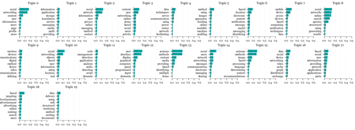
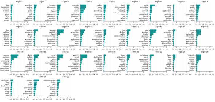
The next attempts used 12, 20, 30 and 45 topics (arbitrary numbers). It was quite hard to conclude which number would work better. With a smaller number, it seemed not sharp enough. As the number of topics grew, they seemed to have become more identifiable as topics (more specific), but my ability to compare how different one topic might be to another decreased, precisely due to the high number of topics. To help me define the most appropriate number of topics, besides printing the score that the top 9 words would get in a given topic (as seen in the graphics above), I also printed to which topic 9 random patent titles would most probably belong. Note that it would be important to look at the a broader spectrum of probabilities per document: imagine that the first topic would score 0.40 and the second would score 0.35. Both topics would be relevant, not only the first. But to keep things simple in the context of this post, I chose to look at one topic only, the one with the highest probability score. You can have a look at the graphics resulting of these attempts, below:

12 topics

Topic-word relationships

Document-topic relationships (9 randomly selected patent titles)

Patent TitleHighest probability

Optimizing retrieval of user interactions for determining contributions to a conversion	Topic 1
Communication based product remarketing	Topic 2
Systems and methods for identifying users in media content based on poselets and neural networks	Topic 4
Systems and methods for incremental compilation at runtime using relaxed guards	Topic 5
Systems and methods for application crash management	Topic 7
Targeting advertisements to groups of social networking system users	Topic 8
Preferred contact channel for user communications	Topic 9
Presence and geographic location notification based on a delegation model	Topic 10
Methods and systems for differentiating synthetic and non-synthetic images	Topic 11

20 topics

Topic-word relationships

Document-topic relationships (9 randomly selected patent titles)

Patent TitleHighest probability

Dynamic identification of other users to an online user	Topic 0
User-specified distribution of stories describing user actions in a social networking system	Topic 3
Search query interactions on online social networks	Topic 8
Communication user interface systems and methods	Topic 12
Systems and methods for determining and providing advertisement recommendations	Topic 15
Social data overlay	Topic 16
Social Networking System Data Exchange	Topic 16
Providing user metrics for an unknown dimension to an external system	Topic 17
Estimating Foot Traffic Lift in Response to An Advertisement Campaign at an Online System	Topic 18

30 topics

Topic-word relationships

Document-topic relationships (9 randomly selected patent titles)

Patent TitleHighest probability

Real-world view of location-associated social data	Topic 2
Search Client Context on Online Social Networks	Topic 3
Using Audience Metrics with Targeting Criteria for an Advertisement	Topic 5
Disaggregation of server components in a data center	Topic 9
Intelligent electronic communications	Topic 13
System and method of detecting cache inconsistencies	Topic 14
System and method for implementing cache consistent regional clusters	Topic 14
Application-tailored object re-use and recycling	Topic 22
Push-based cache invalidation notification	Topic 23

45 topics

Topic-word relationships

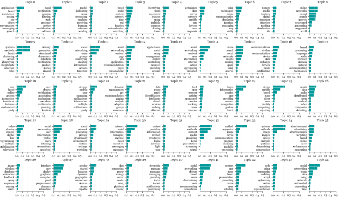
Document-topic relationships (9 randomly selected patent titles)

Patent TitleHighest probability

Intelligently enabled menu choices based on online presence state in address book	Topic 1
Benchmarking servers based on production data	Topic 3
Displaying clusters of media items on a map using representative media items	Topic 6
Subscription groups in publish-subscribe system	Topic 21
Organizing messages in a messaging system using social network information	Topic 30
Bluetooth transmission security pattern	Topic 31
Providing social endorsements with online advertising	Topic 35
Selecting Social Networking System User Information for Display Via a Timeline Interface	Topic 37
Social data overlay	Topic 44

Comments, corrections and tips about this subject, and specifically about the experiments reported above, are more than welcome.

Next

While researching and trying to understand what LDA is and how to use it, I came across a python package called PyLDAvis, which allows the visualization of not only words and documents, but the relationships among them. I also read about the labour intensive and subjective methodology involving the choice of the number of topics in topic modeling, mentioning an evaluation method called perplexity (yet to be added to our glossary). Both are strong candidates as subjects of other posts about topic modeling in this blog. 🙂

Edited in Aug 3, 2018.